In our earlier post, we talked about how the histogram of a black and white picture enabled us to understand the pixel intensity distribution. Furthermore, by equalizing its’ histogram we were able to improve the image’s contrast. Undoubtedly the question is, by examining color image histograms, can we do the same? Different from before, as we will have 3-4 channels in a color image, we need to adapt our approach slightly.
Getting Ready
In order to improve the contrast of a color image, we need to first plot the histogram of a color image. Similar to before, we will import OpenCV and our helper function to display images in Jupyter lab.
import cv2
import numpy as np

#The line below is necessary to show Matplotlib's plots inside a Jupyter Notebook
%matplotlib inline

from matplotlib import pyplot as plt

#Use this helper function if you are working in Jupyter Lab
#If not, then directly use cv2.imshow(<window name>, <image>)

def showimage(myimage, figsize=[10,10]):
    if (myimage.ndim>2):  #This only applies to RGB or RGBA images (e.g. not to Black and White images)
        myimage = myimage[:,:,::-1] #OpenCV follows BGR order, while matplotlib likely follows RGB order

    fig, ax = plt.subplots(figsize=figsize)
    ax.imshow(myimage, cmap = 'gray', interpolation = 'bicubic')
    plt.xticks([]), plt.yticks([])  # to hide tick values on X and Y axis
    plt.show()
Subsequently, we read in our color image.
colorimage = cv2.imread("Hwy7McCowan Night.jpg")
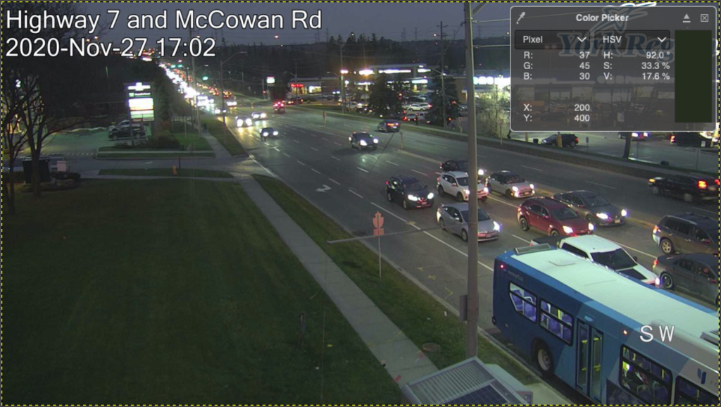
showimage(colorimage)

Color Image Histograms – How to
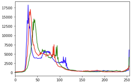
Rather than having only a single channel to process, color images can have 3-4 channels. As a result we need to slightly adjust the approach we took on greyscale images. In order to plot the histogram, we will create histograms for each channel and combine them onto a single plot.
color = ('b','g','r')

#Loop through each color sequentially
for i,col in enumerate(color):

    #To use OpenCV's calcHist function, uncomment below
    #histr = cv2.calcHist([colorimage],[i],None,[256],[0,256])

    #To use numpy histogram function, uncomment below
    histr, _ = np.histogram(colorimage[:,:,i],256,[0,256])

    plt.plot(histr,color = col)  #Add histogram to our plot
    plt.xlim([0,256])

plt.show()  #Show our plot

Equalising a Color Image Histogram
Once we have our color image histogram, we next attempt to equalize each channel. As a result, we hope to achieve a wider distribution and thereby enhance contrast. Since OpenCV’s equalizeHist function only works with a single channel at a time, we quickly apply this function as below.
# For ease of understanding, we explicitly equalize each channel individually
colorimage_b = cv2.equalizeHist(colorimage[:,:,0])
colorimage_g = cv2.equalizeHist(colorimage[:,:,1])
colorimage_r = cv2.equalizeHist(colorimage[:,:,2])

# Next we stack our equalized channels back into a single image
colorimage_e = np.stack((colorimage_b,colorimage_g,colorimage_r), axis=2)
colorimage_e.shape
(540, 960, 3)As shown above, after we equalize each channel, we use Numpy’s stack function to combine them back into our image. In order to verify this was successful, we quickly check the shape of our array.
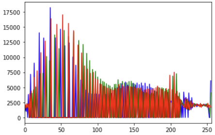
All that remains now, is to quickly plot our new histogram to see what happens after equalization. Finally, we can display the new and old image to verify the results.
# Using Numpy to calculate the histogram
color = ('b','g','r')
for i,col in enumerate(color):
    histr, _ = np.histogram(colorimage_e[:,:,i],256,[0,256])
    plt.plot(histr,color = col)
    plt.xlim([0,256])
plt.show()

# Using Numpy's function to append the two images horizontally
side_by_side = np.hstack((colorimage,colorimage_e))
showimage(side_by_side,[20,10])

Results
Generally, as we compare the old and new image, without doubt we managed to improve the image’s contrast. For instance, notice how the blue bus on the lower right has more distinct border around its’ doors and windows. Additionally, the grass field on the lower left also exhibits more details and texture. These are desired and welcomed results after improving contrast.
Conversely, this approach is not without pitfall. Upon further examination, notice how areas in our original picture that had good contrast now experiences over exposure. For example, the mall on the upper right, or the long queue of cars on the upper left. In essence, we’ve lost certain clarity or information from the image. Finally, notice how the colors didn’t come well together on the upper left. Here we start to see parts of the lawn showing shades of red that weren’t in the original picture.
Even though we’ve managed to improve the contrast of a colored image, it is not without its down sides. Perhaps there is a better way…


