Contours and Hierarchy
When there are many contours or shapes detected in an image, finding which shape to draw the bounding box around can get tricky. Especially in cases when multiple contours, or even contours within contours are detected. Hence understanding the contours and hierarchy will help us better understand the relationship of these shapes.
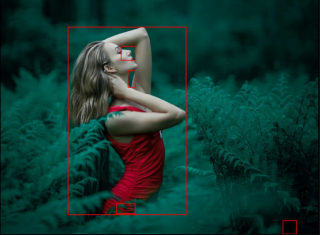
In our introduction to contours and bounding boxes, we made a simple assumption that the subject of our interest is the largest contour. Unfortunately, we can only confirm this assumption after manually inspecting our image. On the other hand, assuming you have a large number of images, inspecting manually is cumbersome. If we look closer at our image, then we find our subject (the lady) is the single largest object. Nonetheless, the relationship between are often interesting. Notice how we have 3 bounding boxes within the largest bounding box (image of lady).

Contours and Hierarchy – Reading the Hierarchy
Previously, we extracted contours and its hierarchy with the below indicated statement. Now we want to look back at the parameters we passed to OpenCV findContours function. Especially what does the “1” represent?
# Generate contours based on our mask
#contours,hierarchy = cv2.findContours(mask, 1, 2)
In fact, apart from passing our mask into the function, the parameters 1 and 2 corresponds to the “Contour Retrieval Mode”, and the “Contour Approximation Method” respectively. Further looking into the “Contour Retrieval Mode”, there are actually 5 out of the box algorithms provided by OpenCV. Previously, when we entered the value 1, we selected the RETR_LIST algorithm. Basically this provides a simple list of all contours in our mask without further relationship details.
print(hierarchy)
[[[  1  -1  -1  -1]
  [  2   0  -1  -1]
  [  3   1  -1  -1]
  ...
  [631 629  -1  -1]
  [632 630  -1  -1]
  [ -1 631  -1  -1]]]
Upon closer examination, the hierarchical details are captured as a list of lists. Each element in the hierarchy corresponds to its corresponding contour and relationship information captured in a 4-tuple. Each element of the tuple tells us:
[NEXT CONTOUR, PREVIOUS CONTOUR, FIRST CHILD CONTOUR, PARENT CONTOUR]
Let us now examine closely at the first two entries in our hierarchy.
Row 0 indicates [1 -1 -1 -1]:
- Next Contour: Contour 1
- Previous Contour: -1 (Doesn’t exist)
- First Child Contour: -1 (Doesn’t exist)
- Parent Contour: -1 (Doesn’t exist)
Row 1 indicates [2 0 -1 -1]:
- Next Contour: Contour 2
- Previous Contour: Contour 0
- First Child Contour: -1 (Doesn’t exist)
- Parent Contour: -1 (Doesn’t exist)
Consequently, you may notice the last two elements in the tuple is always -1 (doesn’t exist). In other words, the hierarchy under RETR_LIST simply lists the contours and doesn’t provide further details in relationships.
Additional Contour Retrieval Modes
As indicated previously, out of the box, OpenCV provides additional contour retrieval modes. All in all, they provide different level of detail on the relationship between contours. Apart from RETR_LIST, there are other retrieval methods:
- 0 = RETR_EXTERNAL
- 1 = RETR_LIST
- 2 = RETR_CCOMP
- 3 = RETR_TREE
- 4 = RETR_FLOODFILL
Interested readers should check out OpenCV Documentation on retrieval modes. Meanwhile, we briefly describe three most commonly used modes:
Because not all applications need the contour hierarchy details, RETR_LIST would suffice.
Meanwhile to get a full relationship between the contours, one should use RETR_TREE. While computationally more expensive, the relationship model is complete. In other words with the additional first child and parent relation. Important to note, depending on our mask the number of contours can be numerous. Due to this, manually reading the hierarchy row-by-row becomes near impossible and perhaps occasionally not necessary.
Another retrieval mode is RETR_EXTERNAL. In this case, findContour builds a list of contour and hierarchy consisting of only the outer most contour. Subsequently, internal contours are ignored and a reduced number is returned. Many times, the reduction in contours improves our ability to identify the object of interest.
Drawing Contours with RETR_EXTERNAL
Chief amongst the benefits of RETR_EXTERNAL is the occlusion of contours within a contour. As was illustrated before, in our original image, we do have large contours within the desired bounding box of the lady. By using RETR_EXTERNAL, we are able to further simplify our picture and remove such child contours. The first step as always, is to import our library and generate our mask using image thresholding.
import cv2
import numpy as np

# Read in our image
reddress = cv2.imread("RedDress1.jpg")

# Generate a mask as before with Image Thresholding
# Convert BGR to HSV
reddress_hsv = cv2.cvtColor(reddress, cv2.COLOR_BGR2HSV)

# Remember that in HSV space, Hue is color from 0..180. Red 320-360, and 0 - 30. Green is 30-100
# We keep Saturation and Value within a wide range but note not to go too low or we start getting black/gray
lower_green = np.array([30,140,0])
upper_green = np.array([100,255,255])

# Using inRange method, to create a mask
mask = cv2.inRange(reddress_hsv, lower_green, upper_green)

# We invert our mask only because we wanted to focus on the lady and not the background
mask[mask==0] = 10
mask[mask==255] = 0
mask[mask==10] = 255
Once our mask is ready, we simply run findContours with RETR_EXTERNAL to get our list. While we could then draw the largest contour, instead we simply plot all contours onto our original image.
# Use RETR_EXTERNAL retrieval mode
contours, hierarchy = cv2.findContours(mask, cv2.RETR_EXTERNAL, 2)

# Use drawContours function to draw the contour
# "-1" in the third arguement can be swapped to draw individual contour
reddress_2 = cv2.drawContours(reddress, contours, -1, (0,255,0), 3)
showimage(reddress_2)


