Skews and Perspectives
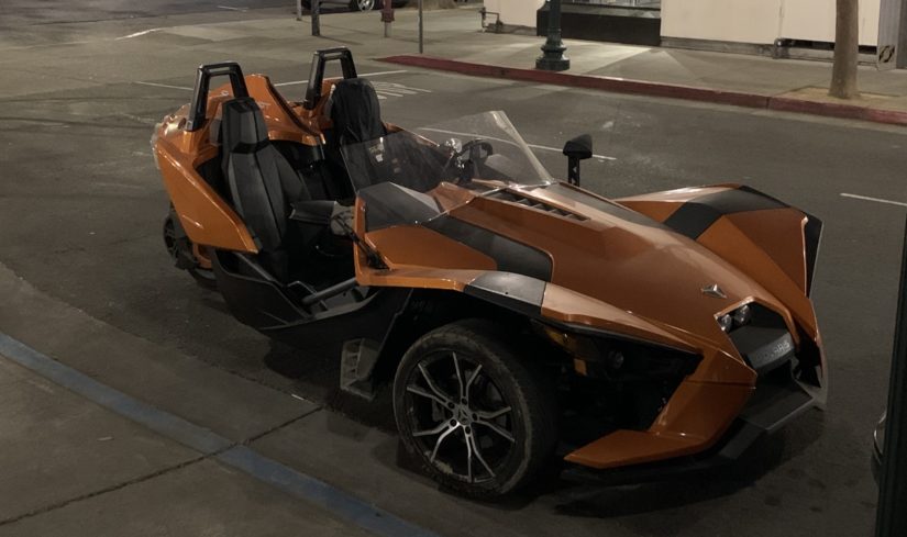
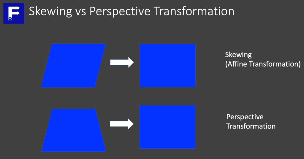
Is that a car or is that a bike? The key is which end are you looking at it. Today we introduce the topic “Skews and Perspectives” on images. Skewing an image is similar but not the same as stretching it. Not only does the image shape or size change in the direction of skewing, but also the intention is to preserve lines and parallelism. Concurrently this may also be referred to as shearing or Affine Transformation.
Perspective Transformation is similar, but instead of perform transformation in 2 Dimensions, we perform the transformation in 3 Dimensions. As a result, one practical use of this, is the ability to re-position images for a more front facing view. To illustrate this better, a simple diagram will directly show what we mean
Skews and Perspectives – Skewing an image
By in large, many times photos we take are somewhat skewed. Particularly as a result of the angle an image is taken. Alternatively we may want to skew our image to give a feeling of “3D”. In any case, OpenCV has built in functions to help us perform this type of geometric transformation (without caring about the math).
Once you have installed OpenCV and other libraries into your virtual environment, we import them and for those working with Jupyter Notebooks, our standard helper function to display images.
import cv2
import numpy as np

#The line below is necessary to show Matplotlib's plots inside a Jupyter Notebook
%matplotlib inline

from matplotlib import pyplot as plt

#Use this helper function if you are working in Jupyter Lab
#If not, then directly use cv2.imshow(<window name>, <image>)

def showimage(myimage):
    if (myimage.ndim>2):  #This only applies to RGB or RGBA images (e.g. not to Black and White images)
        myimage2 = myimage[:,:,::-1] #OpenCV follows BGR order, while matplotlib likely follows RGB order

    fig, ax = plt.subplots(figsize=[10,10])
    ax.imshow(myimage2, cmap = 'gray', interpolation = 'bicubic')
    plt.xticks([]), plt.yticks([])  # to hide tick values on X and Y axis
    plt.show()
First thing to remember when performing skewing is to identify 3 points on our image as an anchor. Furthermore we also need to define where these three anchor points will end up in our transformed image.
#Note: You can use one of your favourite graphic editing software (e.g. MS Paint/GIMP) to identify the points
# 3 Points on the original image
original_pt = np.float32([[390,200],[1650,200],[55,1509]])

# 3 Points on the new image
new_pt = np.float32([[55,200],[1595,200],[55,1509]])
To illustrate this, we show our image after adding the points to our image.
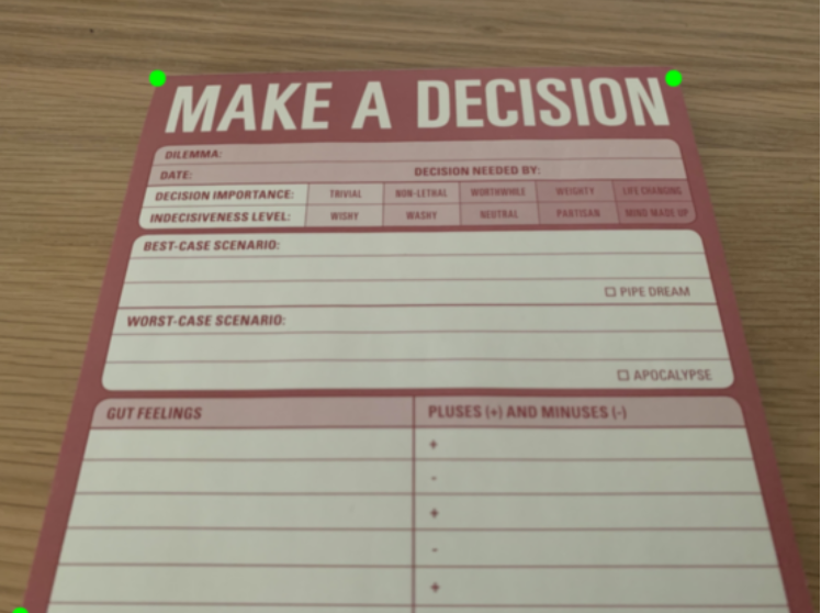
Next we let OpenCV do the heavy lifting in determining the transformation matrix required. Together with our original and new points, we apply getAffineTransform. Then we execute warpAffine based on the transformation matrix we developed.
# Execute getAffineTransform to generate our transformation matrix
M = cv2.getAffineTransform(original_pt,new_pt)

# Feed into warpAffine function to perform our skew
image = cv2.warpAffine(image,M,(image.shape[1],image.shape[0]))
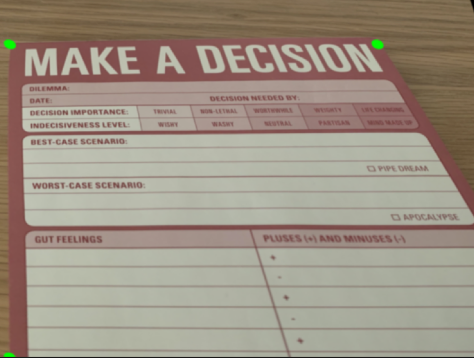
Now that we’ve finished applying the transformation, we simply display our image again to see the results.
showimage(image)
Skews and Perspectives – Perspective Transformation
Now that we’ve seen how to skew an image, we take the next step and show how to perform perspective transformations. In this situation starting with the same image, we would like to better read the text in our image. As can be seen the image was taken at an angle, making text farther away less clear. Consequently if we could apply Perspective Transformation to the image, we could focus on the area of interest.
This time, instead of providing 3 points on the original image and where they should map in the new, we need 4 points.
#Note: You can use one of your favourite graphic editing software (e.g. MS Paint/GIMP) to identify the points
# 4 Points on the original image
original_pt = np.float32([[390,200],[1650,200],[55,1509],[1995,1509]])

# 4 Points on the new image
new_pt = np.float32([[55,200],[1595,200],[55,1509],[1595,1509]])
Afterwards we display our image so you can understand the for points we’ve selected. We’ve deliberately selected the four corners our area of interest. Important to realize, in our new points, they form the corners of a rectangle. That is to say, we want to take the four corners in the picture and map them onto a rectangle. Effectively transforming the perspective.
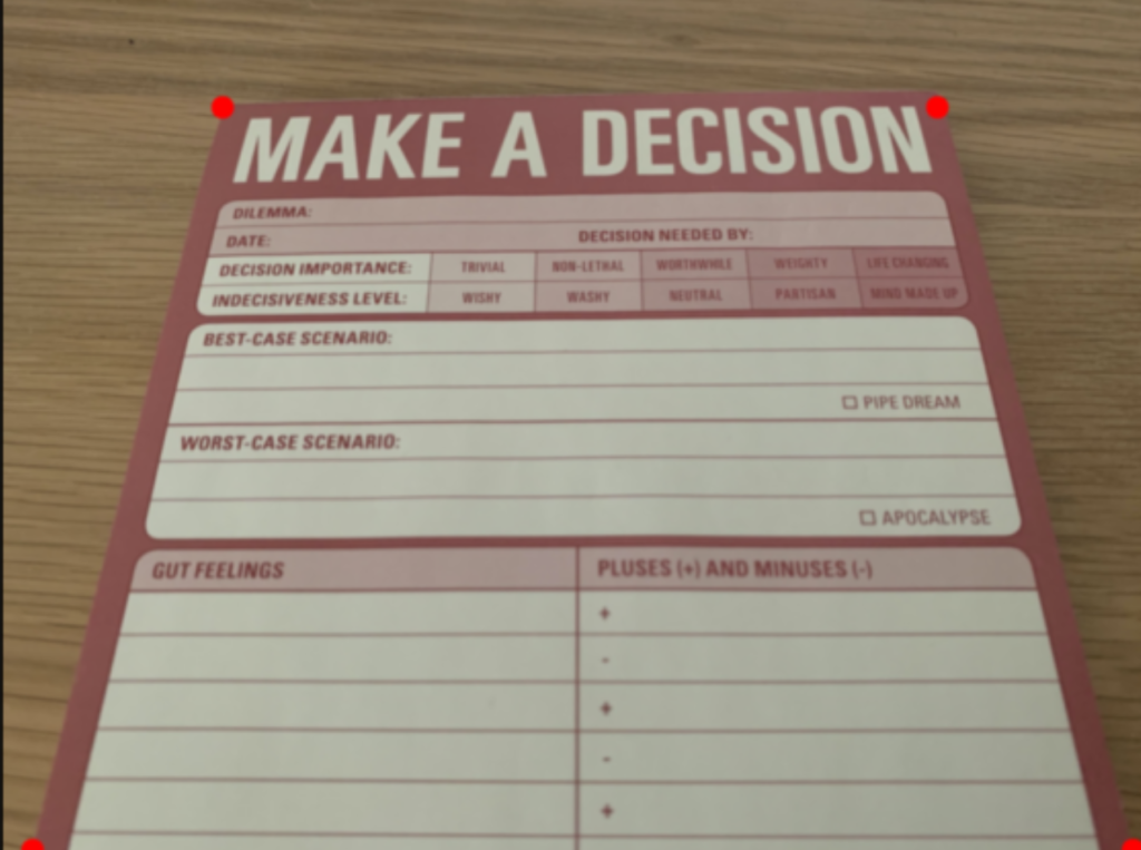
In similar fashion to before, we make use of OpenCV to generate the transformation matrix by using getPerspectiveTransform, then we apply this matrix to the warpPerspective function for processing.
# Execute getAffineTransform to generate our transformation matrix
M = cv2.getPerspectiveTransform(original_pt,new_pt)

# Feed into warpAffrine function to perform our skew
image = cv2.warpPerspective(image,M,(image.shape[1],image.shape[0]))
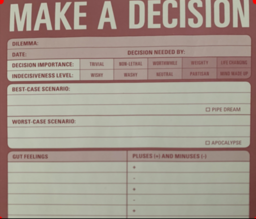
Finally, we can display the results of our input, but more importantly we only wamt the area within our four corners. Hence, we give the range of pixels we are most interested in.
#We display our image by zooming into the new transformed image
showimage(image[200:1509,55:1595])
Summary
In summary, we have quickly demonstrated how we can skew an image or apply perspective transformation using OpenCV. Specifically we looked at how OpenCV can easily help us to generate a transformation matrix. Afterwards how we can apply this on our image. Without doubt, you may ask yourself what would I use this for?
To illustrate, imagine you were building an application to solve Sudoku. In this case, even by taking an image of the grid at an angle, you could transform it as if you took the picture head on. Additionally this would enable more accurate OCR or image recognition routines to run. Therefore, the application in focusing on part of an image you are interested in will be invaluable in further processing steps… Stay tuned.

