Data Wrangling Categorical Data
Once we have cleansed our data, we move on to discuss about Data Wrangling. Data Wrangling is the process of transforming raw data from one form into another format in the intent of making it more valuable for downstream processes such as analytics. Today we will first cover a few commonly used data wrangling techniques with a focus on Categorical Data.
Mapping of Categorical Data
Categorical Data are commonly encountered as part of any dataset. For example, imagine you have a list of movies and you want to group them based on genre. Based on the different type of movies, you may come up with genres such as Action, Horror, Comedy, etc. These different genres are an example of categorical data. To simplify working with categorical data, it is often better to convert them from text into numbers. The reason for this is several fold, on one hand numerical representation are smaller and easier to store. On the other hand it helps relieve different types of spelling/lower case/upper case complications.
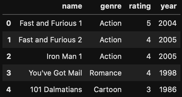
To map into numerical categorical data, we can apply the following code. Afterwards we can easily cast it as a categorical type.
import pandas as pd
movies=pd.read_csv("movies.csv")
movies.genre, mapping = pd.factorize(movies.genre, sort=True)
movies.head()
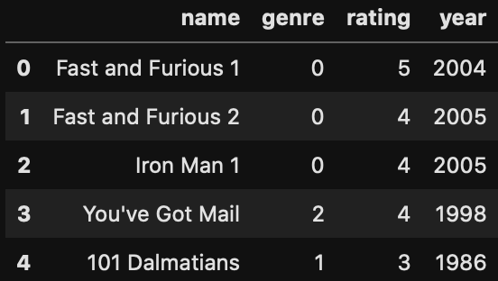
print(mapping)
Index(['Action', 'Cartoon', 'Romance'], dtype='object')
movies.genre = movies.genre.astype('category')
movies.dtypes
name        object
genre     category
rating       int64
year         int64
dtype: object
One Hot Encoding – Low Number of Categories
Another useful way to convert your data into numerical representation is to use one hot encoding. One Hot Encoding is to process of taking categorical values of a column and converting each element as a unique column. Afterwards the value is set to 1 if the column matches the original data. Let’s look at an example based on our movies dataframe.

Notice that the movie rating was created in a numerical format. In order to apply one hot encoding to the rating we execute the command:
rating_one_hot=pd.get_dummies(movies.rating)
We then put this one hot encoded dataframe side by side to our original dataframe so you can compare what has happened.
pd.concat([movies.rating,rating_one_hot], axis=1)

Notice that each unique value in our column “Year” has now been converted into a separate column named after its’ unique value (e.g. 1986, 1998, 2004, etc.). Where the element in the column “year” matches, a value of one is entered, and the remaining columns are zero.
Binning of Values
Even though our data may already be in a numerical format, sometimes it may be in our interest to group them into ranges (or so called bins). Typical examples of binning would be used on datapoints such as age or year. In the case of age, there may be too many columns for one hot encoding, and you rather bin your data into bins of 10. As for year, you may find it is easier to analyze if you binned your data by decade (e.g. 70s, 80s, 90s, etc.). To illustrate how to perform binning, let’s look again at our movies table.

Assume we want to bin the year when the movie was released into 3 equally sized bins. In order to do this, we would issue the following command. We add an addition command to concat the result with our original “year” column side by side for ease of comparison.
year_cut, year_bin = pd.cut(movies.year, bins=3, retbins=True, labels=False)
pd.concat([movies.year,year_cut], axis=1)
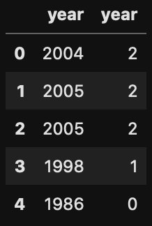
Notice how in the new column, the results returned was an integer ranging between 0 to 2. We’ve also saved the bins themselves within another variable “year_bin”. Hence, we could theoretically lookup the bins for each row by referencing year_bin. So taking the first row of our returned results, the year value of 2 would be between [1998.667 2005].
print(year_bin)
[1985.981 1992.33333333 1998.66666667 2005. ]Summary – Data Wranging Categorical Data
Today we went over three of the basic data wrangling methods for processing categorical data. By converting our dataset into numerical representation, we achieve several benefits such as smaller storage size. But more importantly we have better prepared our data for further analysis techniques such as those required in machine learning models. As a recap, today we looked at how we can:
 | About Alan Wong… Alan is a part time Digital enthusiast and full time innovator who believes in freedom for all via Digital Transformation. 兼職人工智能愛好者,全職企業家利用數碼科技釋放潛能與自由。 |

