Data Cleansing – Missing Data

Data Cleansing – Missing Data

During the process of Data Cleansing you may come across missing data. This happens as a result of different reasons. For instance a power outage leading to an offline sensor for several hours, or a human data entry error. Whatever the reason is, missing data is undesirable as this can skew our analysis or lead to biases. 

As an example, let’s say we wanted to determine the average grade of a class of four students. It would be ideal if all students were present to take the same test. From there we can directly calculate the average. 

import pandas as pd
import numpy as np
myclass=pd.read_csv("Classroom.csv")
myclass['Geography']=[67.0,73.0,49.0,77.0]
myclass.head()

Myclass.describe()

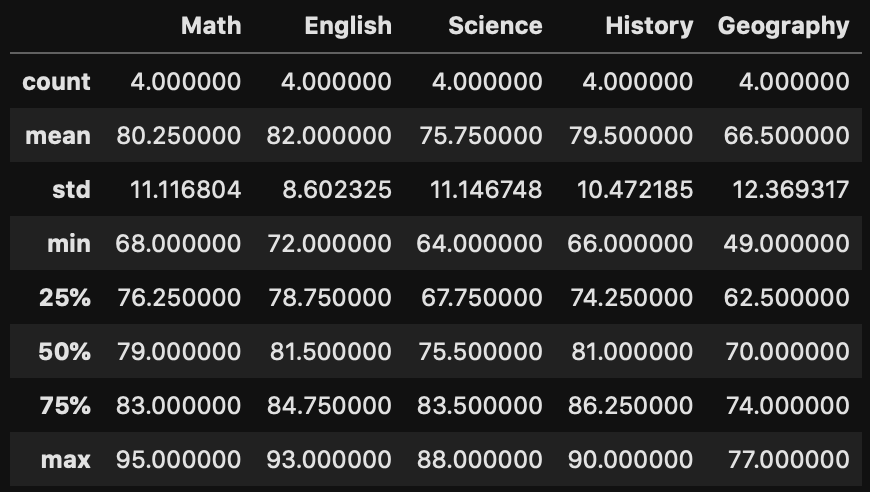
Instead due to illness two of the students didn’t take the geography test, how would this affect the class average?

myclass['Geography']=[67.0,73.0,np.nan,np.nan]
myclass.head()

myclass.Geography.describe()

count     2.000000
mean     70.000000
std       4.242641
min      67.000000
25%      68.500000
50%      70.000000
75%      71.500000
max      73.000000
Name: Geography, dtype: float64

In the example above we can see that when two students missed the test, the average grade in geography was increased from 66.5 to 70. In other words, missing data poses a serious challenge to our data analysis.

Today let’s look at some of the strategies to address this challenge.

Option 1 – Missing Data – Drop Missing Values

The first strategy you can take to address missing values is simply to drop those data points. In other words as we do not have the full set of data, we attempt to avoid any biases in our overall results be excluding them from our analysis.

In our class of four students, we have two options available. Either drop all students who did not take all tests, or drop the geography results in calculating the class average.

myclass.drop(index=range(2,4,1))

myclass.drop(index=range(2,4,1)).describe()

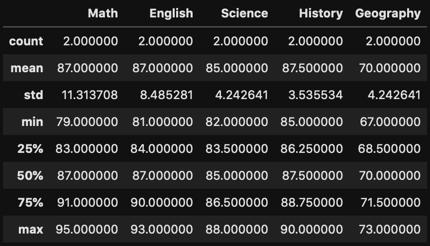
Now that we have dropped the students with missing values, we are able to further determine the class average of the remaining student. It is critical to consider how many data points you have before making any decision to drop datapoints. In our case of four students, dropping two of them represented half of our data and obviously was not the best approach. On the other hand if your dataset contained hundreds or thousands of students, the affects of dropping two are limited.

Option 2 – Missing Data – Averaging

A second strategy for working with missing data is to supplement the missing values with the population average. Once again looking at our class of four students, the idea here is we assume the average of those students who took the test is a good representation of those who did not. In doing so, we would supplement the average geography grade to those who didn’t take the test.

myclass.loc[(myclass.Geography.isna()), 'Geography'] = myclass.Geography.mean()
myclass.head()

myclass.describe()

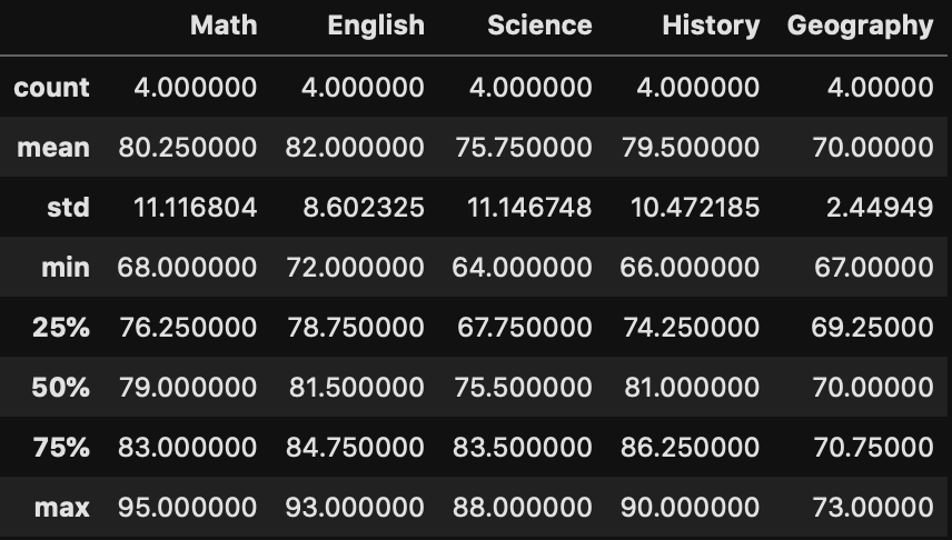
Reviewing our test scores in Geography, notice that we have kept the mean at 70, while the count has remained at 4. In contrast, when we took option 1 (dropping records with missing data), the count was only 2. This approach preserves the mean with a slight sacrifice to the standard deviation. Nevertheless, gives us a good approximation.

Option 3 – Imputation by Last recorded value

Imputation is a methodology to fill in missing values based on closely related data points. Dependent on the type of data we are working with, there could be numerous ways imputation can be performed. One of the simplest way would be to fill the missing values with the last recorded value.

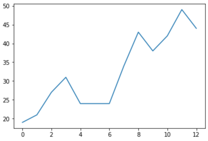
Suppose we have a dataset represented like below with 2 values missing (x = 5 & 6).

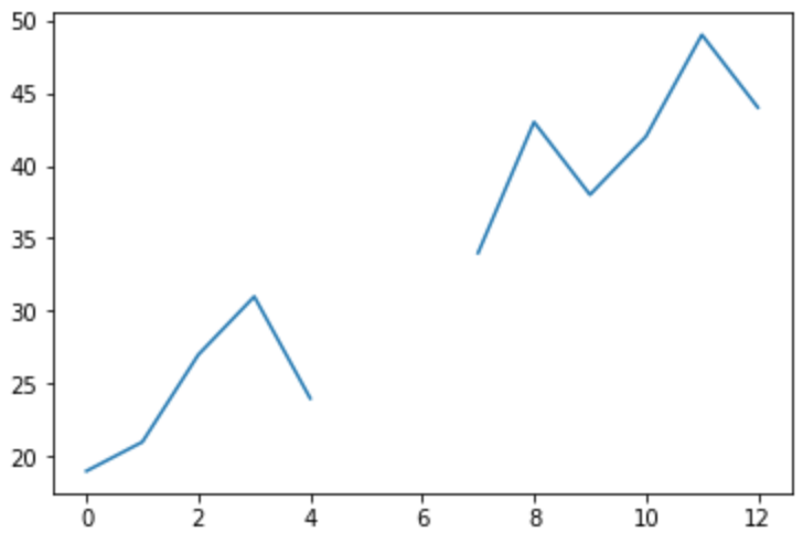
The idea behind supplementing with the last recorded value would be to fill in the values to be 24 (the last known value when x=4). This would result in a chart as below

Option 4 – Imputation by Regression

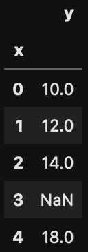
Perhaps a better approach to imputation is to make use of regression to make an educated estimate on what the missing value would be. To illustrate, imagine we have datapoints that locally reflects the relationship y = 2x +10 like such:

series = pd.read_csv("series.csv", index_col="x")
series.head()

plt.plot(series)

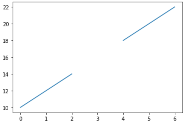
Notice we have a missing value when x=3. The idea behind imputation is to fill in the missing value based on any trend or relationship with nearby values. Performing linear regression of the data points before and after our missing value, we could decide to supplement the the missing value as 16.

Taking an image as another example. We have an image with a time displayed in 12 hour format.

Should some pixel in the RGB space be missing as illustrated below, we could interpolate what are the missing Green and Blue channels from the values from surrounding pixels. A simple approach is to look at the eight pixels directly surrounding the missing pixel. Take an average and supplement the missing details.

Summary

Today we have taken a look into the topic of Data cleansing – Missing Data. This a real world challenge that that all data scientists need to address on a daily basis. We took a brief look into why missing data can be problematic and described several ways one can take to address the issue. Common solutions can range from simply dropping any datapoints with missing data, to more sophisticated approaches such as regression techniques. Do you have other strategies to manage missing data? If so, feel free to leave a comment and share this with us.

If you have not already, check out our other articles on Data Cleansing – Data Types and make sure your data is well suited for analysis

About Alan Wong… Alan is a part time Digital enthusiast and full time innovator who believes in freedom for all via Digital Transformation.  兼職人工智能愛好者，全職企業家利用數碼科技釋放潛能與自由。