Data Wrangling – Data Normalization
The data wrangling – data normalization we want to talk about today is different that what you will find for the top google searches. There, you will most likely find articles about data storage in databases and how to optimize your data. In the past we talked about data wrangling for categorical data, as well as some basic techniques to extract and splice text. Instead, we mean something else when we talk about data normalization in the context of Data Science. Here we refer to the standardizing our dataset into a closer and centered numerical range.
Why is Data Wrangling – Data Normalization beneficial
Even though not all numerical values need to be normalized. This should be determined based on the nature of the dataset. Often times it may become beneficial to do so. As an illustration, suppose we wanted to analyse the Toronto housing price and had two values for each housing unit; Age and the Price. Accordingly we can imagine most housing unit age falls within the range of 0 – 100 years. Meanwhile the price of the unit can range anywhere from 300,000 to to 5,000,000. Comparatively we can see the numerical range and average for price is much higher and wider than the age. In this case if we do not perform normalization of our data, the weights of the housing price will dominate over age. This is due to the higher variability of housing price.
Standardising of numerical data
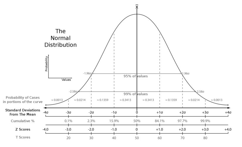
Now let us see how this is done. In order to calculate the normalized value or also referred to as the standard score (or Z-score), we employ the formula:

To show this in action let us look at some basic code.
import pandas as pd

housing = pd.read_csv("Housing.csv")
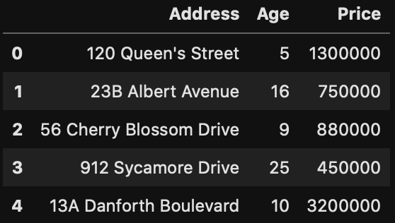
housing.head()

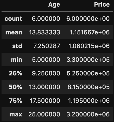
housing.describe()

In particular notice how the mean and standard deviation of Price is much larger than Age. What this means is, the Price will easily outweigh the Age since the values and range are much higher. In order to normalize our value we would need to:
housing['Norm_Age']=(housing['Age']-housing['Age'].mean())/housing['Age'].std()
housing['Norm_Price']=(housing['Price']-housing['Price'].mean())/housing['Price'].std()

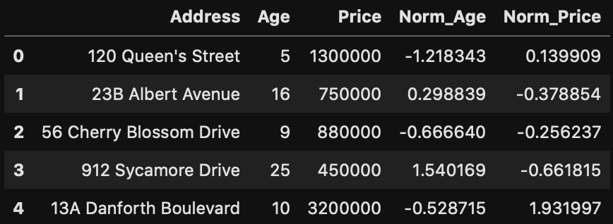
housing.head()

In this situation, see how we managed to normalize the value around zero, and preserve the relative distribution. As a result, our normalized values for Price will not overweight our Age values.
Standardising Images
Recall in our earlier article on Reading in Data that image data in the RGB colour space is a value between 0-255. There are benefits to scale down this range between zero and one. Since we are working with a mix of RGB color, larger values should not out weight smaller values. As an example, black would be (0,0,0), but does be less impactful than white (255,255,255). Therefore normalising the RGD channels will assist our image analysis in the future.
from PIL import Image
import numpy as np
# Convert out image into a numpy array
img = Image.open('Food.JPG')
array = np.array(img)
print(array.shape)
(2160, 3840, 3)
print(array[0])
[[ 43  47  58]
 [ 51  55  66]
 [ 50  54  65]
 ...
 [145 131 130]
 [150 136 135]
 [150 136 135]]
norm_array = array / 255
print(norm_array[0])
[[0.16862745 0.18431373 0.22745098]
 [0.2        0.21568627 0.25882353]
 [0.19607843 0.21176471 0.25490196]
 ...
 [0.56862745 0.51372549 0.50980392]
 [0.58823529 0.53333333 0.52941176]
 [0.58823529 0.53333333 0.52941176]]
Summary
In conclusion we looked into why we would normalise our data. It is to prevent the over-powering of numerical datasets with high variability over those with less. In addition we talked about how to calculate the standard or Z-score for numerical data as well as how to normalize image data.


