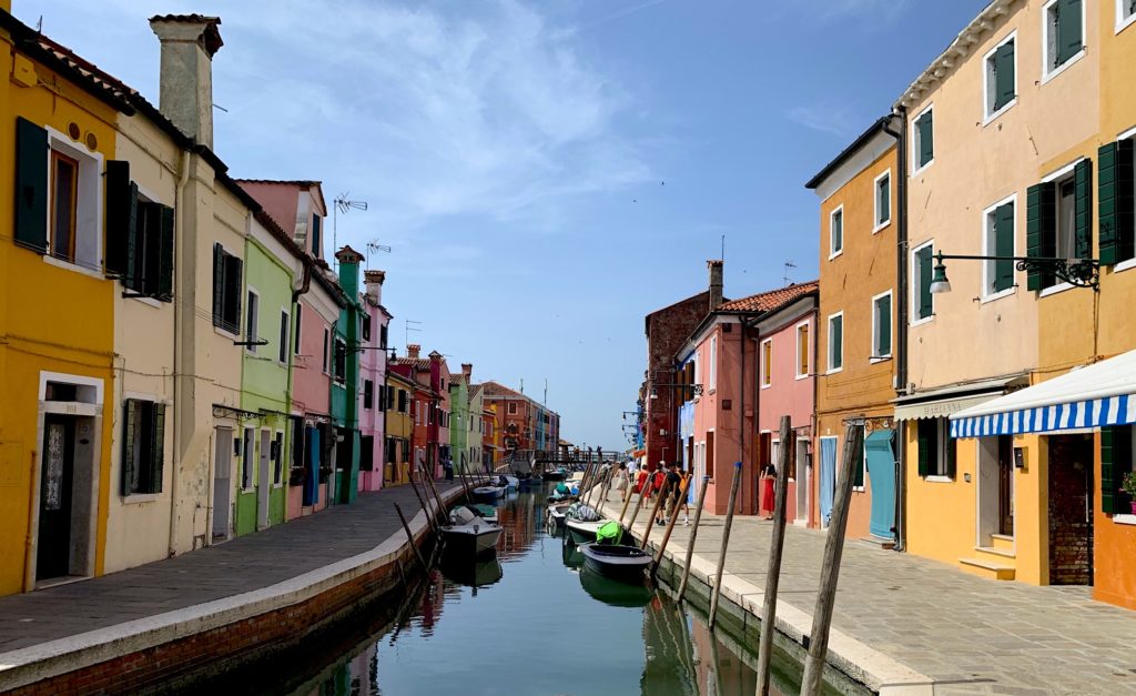
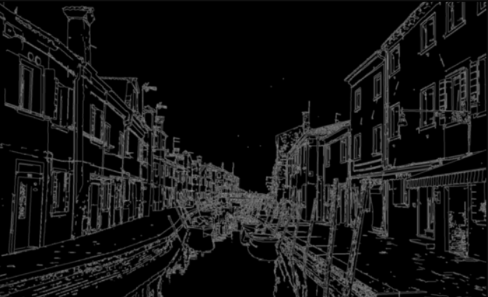
Canny Edge Detection is a method to identify edges of objects within an image. Consequently today we would like to introduce how you can apply this technique using OpenCV and Python. Doing so, you can simplify features in an image and prepare for further image processing like image segmentation. Recall our previous article on contours and hierarchy. If we first performed edge detection, then we could also reduce the number of contours for more accurate results. Subsequently, drawing bounding boxes based on contours can also be simplified and improved. Hopefully, I’ve convinced you of just some of the many practical applications. Let us now see how we can do this.
Background – Concepts of Canny Edge Detection
Generally in our blogs, our intention is not to explain the mathematical theories behind how or why certain concepts work. Instead we will briefly describe its’ concept so you get a basic understanding. Interested readers can refer to the original paper – A Computational Approach to Edge Detection). In short, the Canny Edge Detection method is a multi-step process. While OpenCV provides a very simple function to simply how to perform this, the steps are as follows:
- Smoothen the image. Firstly the image goes through noise reduction. Anyone who has taken photos in a dark area or with high ISO settings can relate. Difference in contrast and color may be wrongly highlighted as edges in noisy images.
- Determine the intensity of the gradient. Determine the gradient of each pixel along both vertical and horizontal axis. The larger the difference between pixels, the larger the gradient.
- Local area check. Compare the gradient of a pixel to its neighbors along each axis. Only one edge exists amongst pixels in next to each other. When comparing the gradient against neighboring pixels, the one exhibiting the highest gradient is the edge. In turn, the others are suppressed.
- Thresholding. Finally, we use a minimum and maximum threshold to decide whether the remaining pixels are on an edge or not. Pixels gradients above the max threshold are edge pixels. Likewise, pixel gradients below the min threshold are not edge pixels. Lastly, we further evaluate pixel gradients falling between the threshold. If they are next to an edge pixel, then they are also edge pixel.
Practical application in OpenCV
Straightaway when using OpenCV, we import the OpenCV libraries and define our helper function. As we use Jupyter notebooks, this helps to display our images inline with matplotlib.
import cv2
from matplotlib import pyplot as plt

#The line below is necessary to show Matplotlib's plots inside a Jupyter Notebook
%matplotlib inline

from matplotlib import pyplot as plt

#Use this helper function if you are working in Jupyter Lab
#If not, then directly use cv2.imshow(<window name>, <image>)

def showimage(myimage, figsize=[10,10]):
    if (myimage.ndim>2):  #This only applies to RGB or RGBA images (e.g. not to Black and White images)
        myimage = myimage[:,:,::-1] #OpenCV follows BGR order, while matplotlib likely follows RGB order

    fig, ax = plt.subplots(figsize=figsize)
    ax.imshow(myimage, cmap = 'gray', interpolation = 'bicubic')
    plt.xticks([]), plt.yticks([])  # to hide tick values on X and Y axis
    plt.show()
Subsequently, we import our image
myimage = cv2.imread("Burano1.jpg")
showimage(myimage)

Using OpenCV’s built in Canny Edge function, we define our min and max threshold. Afterwards we feed our image into the model to obtain the results
# We use the built in Canny Edge function from OpenCV to find edges
# Three parameters are needed to execute the Canny Edge function
# Image, Min Threshold, Max Threshold

min_interval = 120
max_interval = 250

# Create a new image of the edges
image_edge = cv2.Canny(myimage,min_interval,max_interval)
Finally we display our results.
showimage(image_edge)

Summary
In reality, with OpenCV’s built in function, it is very simple to apply Canny Edge Detection. Evidently objects that are more uniform in color and have high contrast to the adjacent objects are processed better. Therefore you can easily see the outlines of the buildings in our image. Furthermore the edges of the white and blue podium on the right was impressive. Undoubtedly this is because the strips exhibited a high contrast. On the other hand, look closely at the wooden piers. When wood grains and shadow have a smaller contrast, the edge detection wasn’t clean. Whereas tuning our min and max interval might help, perhaps there are other edge detection techniques?


