Opening and Saving Images
Opening and saving images is the most fundamental operation needed when working with images. Accordingly our article here will guide you on how to perform these basic operations as we dive deeper into image processing. At first it should be pointed out that there are many libraries and ways to read in image data. In fact, we have covered one approach before in our earlier article on Reading in Data. Explicitly we will be working with a common image library called OpenCV. Opening and saving images with OpenCV becomes very easy to manage. By and large OpenCV stands for Open Source Computer Vision and includes many useful features that we will discuss later.
Opening and Saving Images with OpenCV from disk
Our computers and smartphones contain many images and photos we have taken or were shared with us via social media. Occasionally one may find the need to edit these photos (such as resizing or rotating an image). Especially, if you have many photos that need to be processed like from a recent vacation, doing so manually can be cumbersome. In this case, wouldn’t it be great if we could programmatically process images? As a result the first thing to know is how to read in a saved image.
import cv2

#Reading in a color image
image_bgr = cv2.imread("Phone.jpg")

#Reading in an image and converting to black and white
image_grey = cv2.imread("Phone.jpg",cv2.IMREAD_GRAYSCALE)
However, reading in an image to our system is not enough. Undoubtedly it would be even better if we are able to view the image as well.
#Normally if we wanted to show in image within our Python code, we could directly use
#the cv2.imshow(<Window name>, <image>) function provided by OpenCV

cv2.imshow("Our image", image_bgr)
cv.waitKey()  #This tells the OpenCV to wait for a key press and keep the image on screen
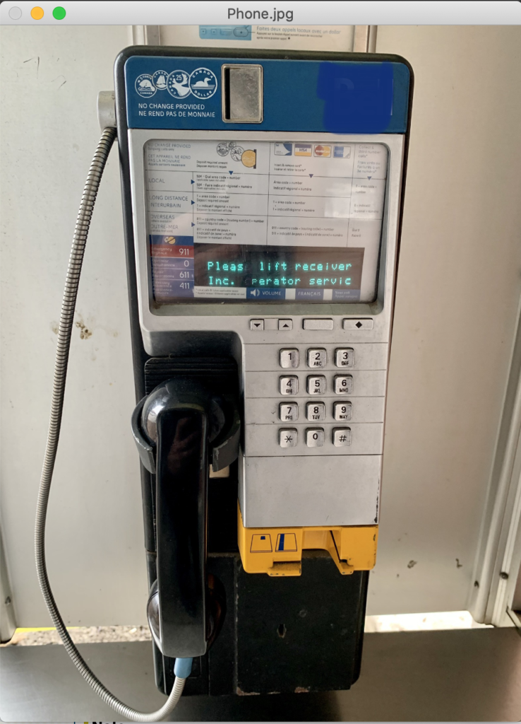
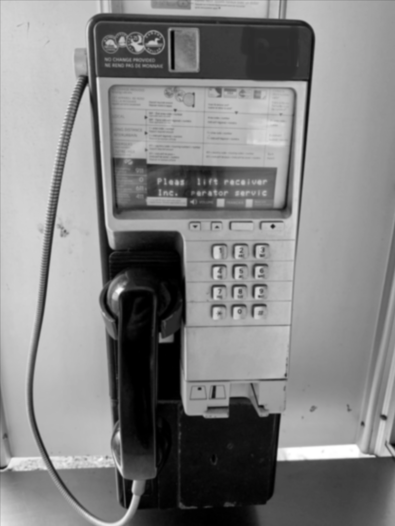
While the above approach will work in Python, if you are you building your code within a Jupyter Notebook, you will find this crashes. In order to work around this, we instead once again leverage Matplotlib to assist us to display inline images. To begin, we start with displaying our greyscale image, followed by our colored version.
#The line below is necesary to show Matplotlib's plots inside a Jupyter Notebook
%matplotlib inline
from matplotlib import pyplot as plt

#We first plot our greyscale image
fig, ax = plt.subplots(figsize=[10,10])
ax.imshow(image_grey, cmap='gray', interpolation = 'bicubic')
plt.xticks([]), plt.yticks([])  # to hide tick values on X and Y axis
plt.show()
#We then plot our color image
fig, ax = plt.subplots(figsize=[10,10])
ax.imshow(image_bgr)
plt.xticks([]), plt.yticks([])  # to hide tick values on X and Y axis
plt.show()
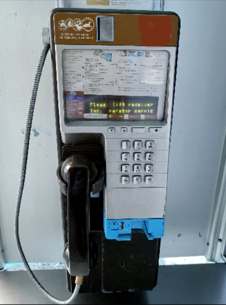
Notice that while we were able to display our image, the colors seem to be wrong. This is because within OpenCV, images are read into an Array as BGR. This means the first column of the array represents Blue, the second Green, and the last Red. On the other hand, Matplotlib expects colors in the array to be depicted in RGB. As a result, we need to simply reorder the columns of our image array into RGB and then display our image again. In order to help us, we’ve built a small function that will do this for us.
def showimage(myimage):
    if (myimage.ndim>2):  #This only applies to RGB or RGBA images (e.g. not to Black and White images)
        myimage2 = myimage[:,:,::-1] #OpenCV follows BGR order, while matplotlib likely follows RGB order

    fig, ax = plt.subplots(figsize=[10,10])
    ax.imshow(myimage2, cmap = 'gray', interpolation = 'bicubic')
    plt.xticks([]), plt.yticks([])  # to hide tick values on X and Y axis
    plt.show()

showimage(image)

Basic Information about an Image
Besides the ability of viewing, some basic information about our image may prove important to understand. For example, one could be interested to know the size of our image, or the BGR values at a specific pixel. Additionally how could I view only a certain portion of my image.
# Understanding image size
image_bgr.shape
(2100, 1575, 3)
# Accessing individual pixel information
# The following command returned by BGR values at pixel 500,500
image_bgr[500,500]
array([164, 169, 170], dtype=uint8)
# We can also display parts of an image by simply providing the pixel range we are interested in
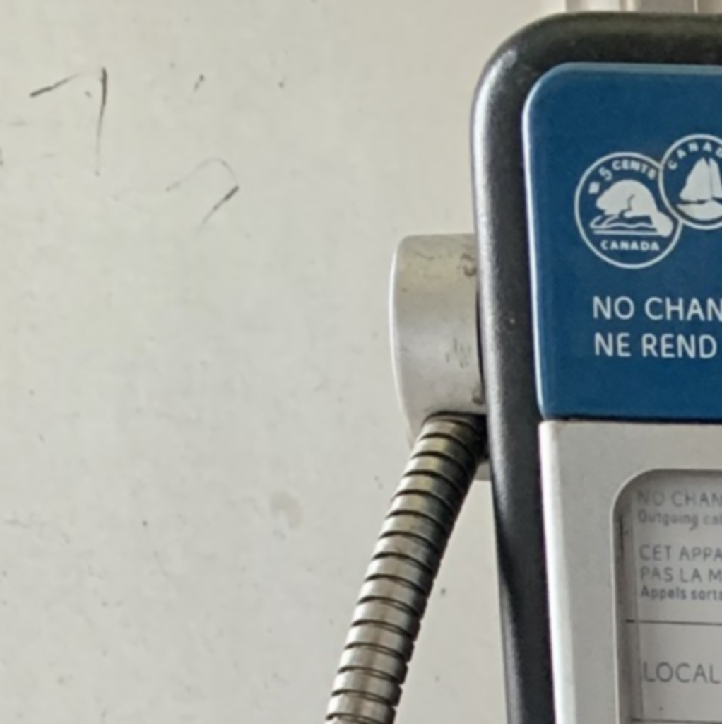
showimage(image_bgr[50:500,50:500])
Opening and Saving Images with OpenCV from camera
Even though having access to images on disk is handy, occasionally we may find capturing images live from a camera is needed. In order to do this, we introduce a new object in OpenCV called “VideoCapture”. Instead of opening an image object, we make a connection to a camera (e.g. webcam), capture the image, and release our control over the camera.
#Depending on your machine, you may have one or more cameras
camera = 0  # 0 is the default camera

#Open our video feed
cap = cv2.VideoCapture(camera)

#Capture an image from our camera
frame_opened, image = cap.read()

#Close our video feed
cap.release()
Finally, once we have captured our image, saving this back to disk is as simple as running a single lines of code.
# The below code helps us to save our image
# The first parameter is our file name. Note the file extension tells OpenCV which image format to use
# The second parameter is the image we want to save
cv2.imwrite("Webcam Photo.jpg",image)
Summary
Summing up, in this article we revisited the most fundamental aspect of working with images; namely opening and saving images. In order to further perform image processing, being able to do so is of utmost importance. Subsequently, we started briefly to think about colorspace; a topic we will further look into in the future. Not to mention, we also for the first time saw how we can capture images from a connected camera. Of course, this is only the beginning, stay tuned for our further articles on how we can process images.

